Results
I split my findings into two parts. First, real-world evidence from public data that I can stand behind right now. Second, the analysis framework I built and validated for the field data I still have to collect.
Part 1 · Real-world evidence real data
Where the species actually occur
I pulled 1,402 georeferenced records of my four species from GBIF across northwest and central Connecticut, from the Litchfield hills east to the Farmington Valley. The records cluster around towns, roads, and trails.
real data Interactive map of 1,402 GBIF records by species (points cluster when zoomed out). Click any point for species, year, and source; toggle the density heatmap or switch to satellite. Open the full map (all layers) →
Real clusters (Getis-Ord Gi*)
When I grid the records into 1 km cells and run Getis-Ord Gi*, each species shows statistically significant clusters. Japanese knotweed forms a clear hotspot along the developed Torrington corridor. I also include the all-species map as an honest control for where people tend to look.
real data Interactive Getis-Ord Gi* hotspots (red cells) with a monitoring-priority layer. Turn the species points on or switch the basemap. Hover a cell for its record count. Full map →
Local patterns
Visible reporting clusters appear in several developed-edge landscapes, including parts of the Farmington Valley, Greater Hartford, and northwest Connecticut. These clusters should be interpreted carefully because public records can reflect where people observe and report plants.
Still, the patterns help identify useful places for local monitoring, education, and field validation.
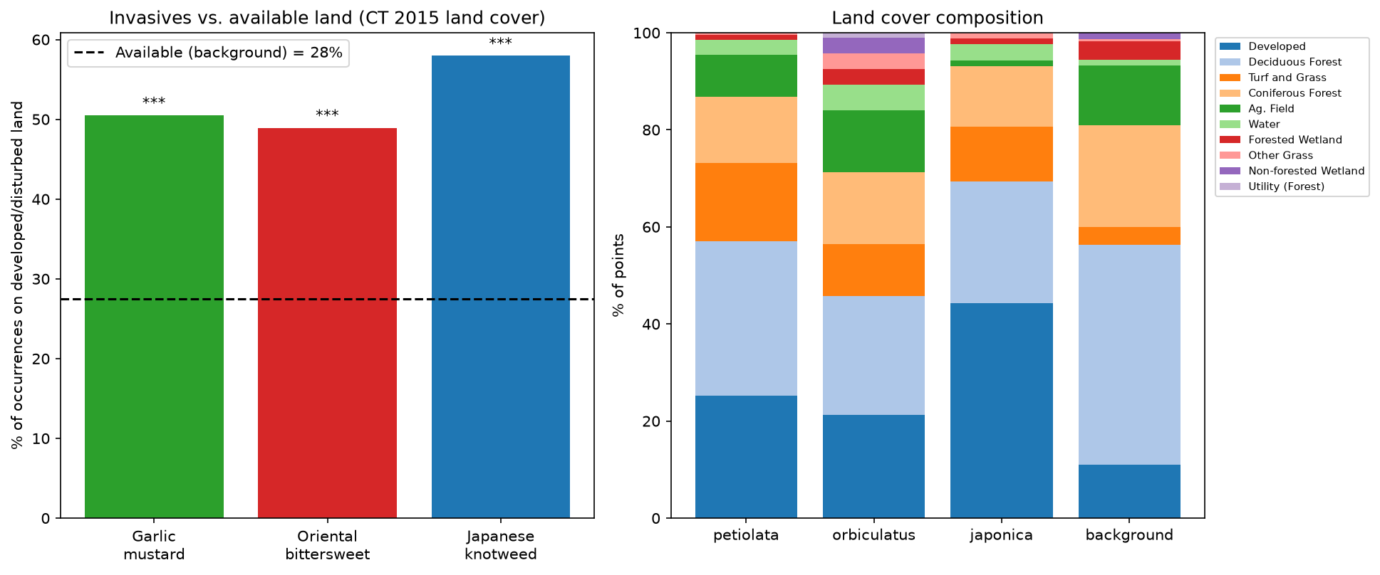
Most invaders sit on disturbed land more than chance
This is my central real-data result. I sampled CT ECO 2015 land cover at each occurrence and at random background points. The land itself is only 29.8% developed/disturbed, and three of the four species turn up there far more often. Japanese barberry is the exception, for a reason I return to below:
| Species | Records | On disturbed land | Selection ratio | p-value |
|---|---|---|---|---|
| Japanese knotweed | 196 | 58.7% | 1.97× | 2 × 10⁻¹¹ |
| Oriental bittersweet | 209 | 56.9% | 1.91× | 1 × 10⁻¹⁰ |
| Garlic mustard | 523 | 51.6% | 1.74× | 4 × 10⁻¹¹ |
| Japanese barberry | 269 | 30.5% | 1.02× | 0.91 (n.s.) |
How close to development? real data
Barberry looked harmless in that first test only because it is a forest-understory shrub: at any given point it usually sits under tree canopy, not on pavement, so a land-cover-at-the-point test cannot see its link to disturbance. A cross-check with 10 m Google Dynamic World (2025 to 2026) said the same, with knotweed, bittersweet, and garlic mustard well above the landscape average (2.5×, 1.9×, 1.9×) and barberry not.
So I asked a sharper question: not whether a plant is on developed land, but how close it is. I measured each occurrence's distance to the nearest built pixel and compared it to random background points. Now all four species, barberry included, are significantly closer to development than random:
| Species | Median distance to built | Within 100 m | p (closer than random) |
|---|---|---|---|
| Japanese knotweed | 54 m | 62% | 4 × 10⁻²⁶ |
| Garlic mustard | 80 m | 55% | 9 × 10⁻³⁸ |
| Oriental bittersweet | 125 m | 46% | 2 × 10⁻¹⁵ |
| Japanese barberry | 198 m | 32% | 6 × 10⁻⁸ |
| Background (random) | 385 m | 21% | n/a |

Predicting relative invasion risk real data
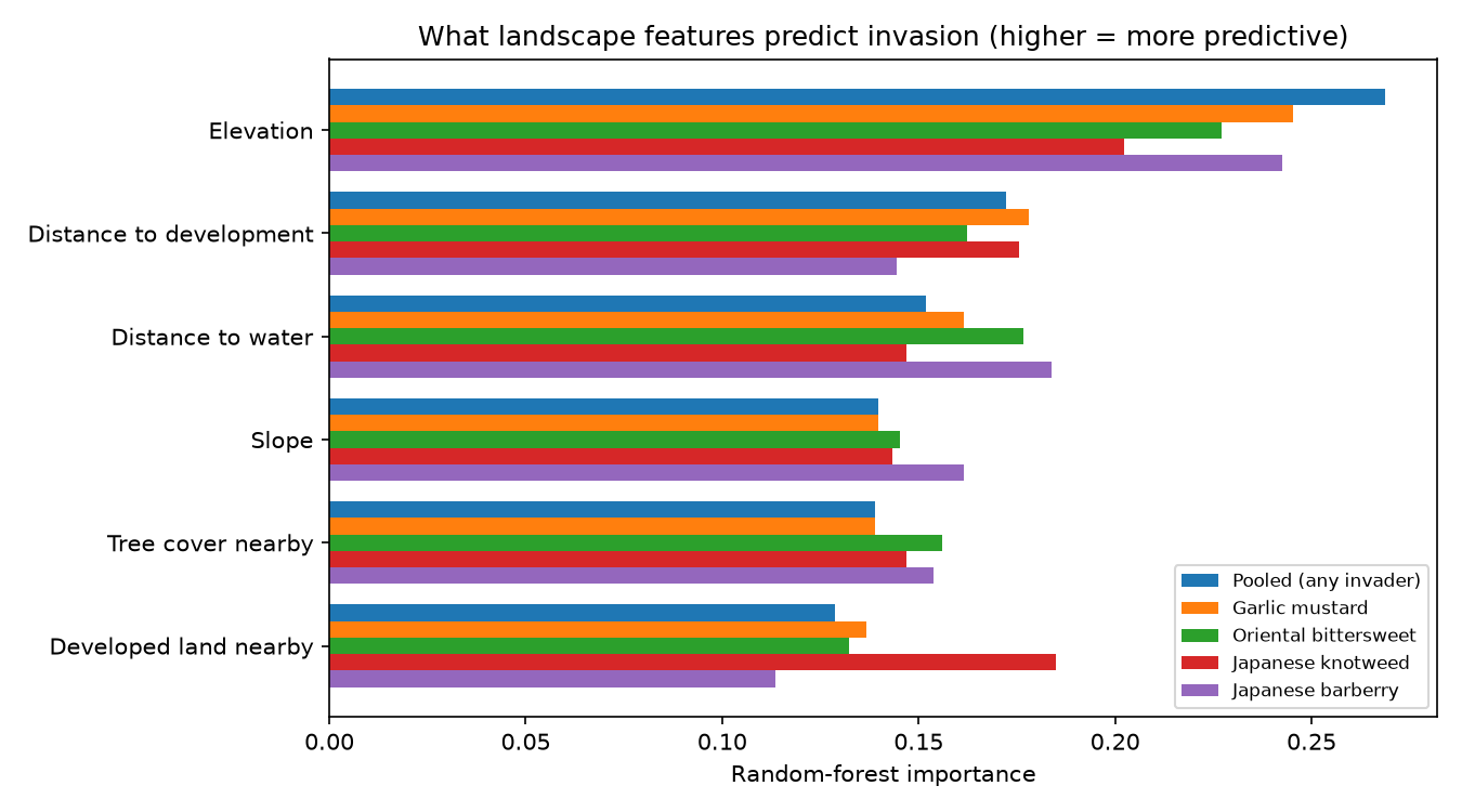
Finally, I pulled the pieces together into a model. I trained a random forest to tell invasive-occurrence locations apart from the average landscape, using six landscape features, and had it map relative invasion risk across the region. Scored honestly with 5-fold cross-validation, the pooled model reaches an AUC of 0.79 (0.60 to 0.70 per species), so it discriminates reasonably well.

The model also ranks which landscape features matter most:
| Landscape feature | Importance (pooled) |
|---|---|
| Elevation | 0.27 |
| Distance to development | 0.17 |
| Distance to water | 0.15 |
| Slope | 0.14 |
| Tree cover nearby | 0.14 |
| Developed land nearby | 0.13 |
Field check: does the map hold up on the ground? real data
Everything above uses public data. To see whether it holds up, I went into the field and recorded 64 of my own occurrences, each with a photo and a GPS point (collected through two of my own submission forms). This is a real ground-truth of the model, focused on the Farmington Valley.


Then the key question: does the model predict higher invasion risk where I actually found invasives? It does, clearly.

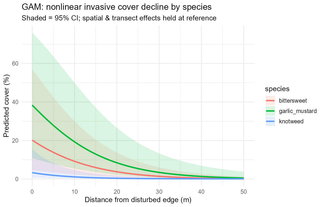
This validates the model. The other half of my plan, a belt-transect test of how cover falls with distance from an edge, needs quadrat measurements I have not entered yet, so the figures in the next section are still a simulated framework.
Part 2 · Analysis framework illustrative, simulated
The edge gradient is nonlinear and species-specific
Different species cluster in different places

From hotspots to a priority map

Conservation priorities
Putting both parts together, and taking into account expert feedback on this project, my recommendations for the study area are:
- Watch the edges and act early. Roads, trails, and field margins are where new patches turn up first, so early detection there is cheap and effective.
- Make protecting intact forest the priority. The interior, like Great Mountain Forest, shows lower invasion. Keeping it that way by stopping spread from the edges is often more valuable than fighting the biggest existing stands.
- The worst infestations are not always the best places to treat. Where invasives have already outcompeted the natives, removing them, even with replanting, often just lets similar or worse invaders move back in, unless there are resources for several years of repeat treatment. In those places effort usually goes further on preventing spread into cleaner ground and on easing the conditions (disturbance, canopy gaps, altered soil) that let invasives win in the first place.
- Target control species by species. Because the invaders occupy different parts of the landscape, a single "invaded zone" approach would miss most of the problem.